Better Cold-Start Forecasting with Nori: New and Short-History SKUs

The cold-start problem

New products are the hardest thing to forecast, because they have no sales history to forecast from. Products with only a few months of sales have the same problem to a lesser degree: a few noisy months isn't enough to separate trend, seasonality, and level.

Why it has been hard

The reason is simple. The per-series models most teams run (ARIMA, ETS, Prophet) are fit one per product, so each one only ever sees that product's own sales. Two years of sales and it can separate trend from seasonality. Two months and it is mostly fitting noise. None at all and there is nothing to fit, so the forecast falls back to a manual guess or a category average. What would actually help, how comparable products behaved when they launched, sits in series the model never looks at.

Throughout this post we use the public Online Retail II dataset (UCI): two years of a UK online gift retailer, with products that first appear on different dates, so it has genuine new and short-history products. Demand is strongly seasonal (a gift shop peaks at Christmas), which sharpens the problem, because a product launched in autumn has no December of its own to learn from.

How Nori changes it

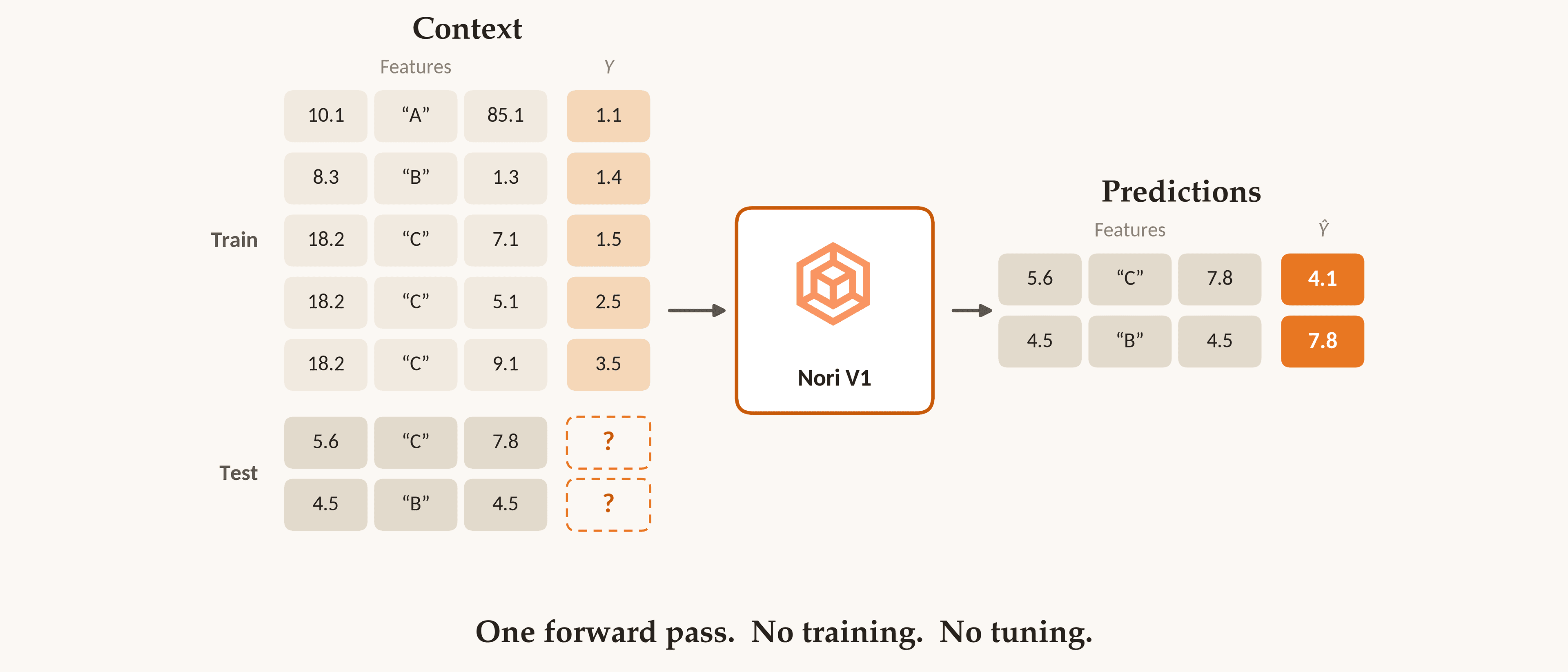
Nori reads the whole catalog at once, so a product with no past of its own can be forecast from the products it resembles. It is a tabular foundation model that does regression by in-context learning: you give it a table of examples at inference time and it predicts the unlabeled rows, with no training step and no per-product fitting. Nothing about the new product changed. What changed is that the other products are in the table with it.

The call to Nori is two lines. You pass the labeled rows as context and the unlabeled rows as queries:

1from synthefy_nori import NoriRegressor
2
3model = NoriRegressor(model="nori-6m")
4model.fit(X_context, y_context)      # labeled rows (established + the new product)
5predictions = model.predict(X_new)   # unlabeled rows (the months to forecast)

There's no training step here. With XGBoost you'd fit a model on the catalog, tune hyperparameters, and retrain whenever the data changes. With SARIMAX you'd fit a separate model per product, which for a brand-new one means you can't even start. Nori skips all of that: the labeled rows are the model's context, not its training data, so adding a new product or a new month of history is just adding rows to the table.

The call never changes. Every decision that affects forecast quality has moved into X_context instead: which rows you hand Nori, and which columns describe them.

Building the context

Because Nori learns from the rows you give it at inference time, improving a cold-start forecast is less about model tuning and more about what you put in the table. This is the tabular equivalent of context engineering for LLMs: you're optimizing the input, not the model. The better the context rows represent the new SKU's situation, the better the prediction.

Good demand planners have been doing exactly this for decades, without calling it that. The discipline has a whole toolkit for the no-history problem: forecast the item from its attributes instead of its past, since pack count, price tier, and design theme are known on day one; borrow a launch curve from how comparable products ramped over their first few months; net out cannibalization when a new variant eats a sibling's volume; scale by planned distribution, because demand follows how many stores actually stock the product. Every one of those is a claim about which products a new SKU should be read alongside — and every one is a column you can put in the table.

X_context starts as the pooled table from above, one row per (SKU, month) with every product in the catalog stacked together, and then gains a column per feature. A new SKU's own history is nearly empty, so the features that carry its forecast have to describe the products it resembles instead. We build them in two blocks.

Category and calendar features

These two blocks are the cold-start enabler: the calendar features are properties of the date, and the category features come from the SKU's neighbors, so both are fully populated for a product with no history of its own.

1# `rows` is the monthly panel joined to its per-category aggregates, which are
2# already shifted so a row only ever sees earlier months.
3rows = panel.merge(category_monthly, on=["category", "month"], how="left")
4by_sku = rows.groupby("sku")
5
6# ---- calendar: properties of the date, so known for any row, cold or not ----
7m = rows["month"].dt.month
8feat["fcst_month_sin"] = np.sin(2 * np.pi * m / 12)   # Dec and Jan are neighbors,
9feat["fcst_month_cos"] = np.cos(2 * np.pi * m / 12)   # not 12 apart
10
11# ---- category: years of history even when the SKU itself has none ----
12feat["cat_units_lag1m"] = rows["cat_units_lag1m"]     # the category last month
13feat["cat_units_lag12m"] = rows["cat_units_lag12m"]   # the seasonal anchor
14feat["cat_yoy_lagged"] = rows["cat_yoy_lagged"]       # growing or shrinking
15
16# a cold SKU has no price history, so this falls back to the category median
17feat["price_vs_cat_lagged"] = (by_sku["avg_price"].shift(1)
18                               / rows["cat_price"]).clip(0.2, 5.0).fillna(1.0)

Own-history features (1+ months of history)

Once a SKU has a month of sales its own past becomes usable: demand 1, 2, 3, 6, 12 and 13 months back, a trailing three-month mean, a year-over-year ratio, and a seasonal-naive forecast built from the last two. Four launch-and-maturity columns (months_since_launch, launch_units, peak_units_lagged, cat_share_lag1m) fill in alongside them. All of it is computed in log-ratio space (log1p(units) - log1p(scale)), so a 10-unit SKU and a 10,000-unit SKU produce comparable values. For a cold row every one of these is zero, which is why the category and calendar columns have to carry the forecast.

Stacking the blocks, then predicting

Stack the two blocks horizontally and that is X_context: 25 columns, one row per (SKU, month), every product in the catalog in the same table. Nori forecasts from it as it stands.

XGBoost needs a tuning step first, because a foundation model beating an untuned GBDT would not be worth writing about. We searched a 576-config grid on an earlier window, so the test months never inform the choice, and a well-regularized default turned out to be hard to beat. That default is the baseline we report; the notebook has the search.

The split is by date, not by row sampling: everything strictly before the forecast month is context, and the forecast month itself is what you ask for. Both models get the same columns, the same rows and the same split. One stores the table and reads it; the other fits parameters to it.

Proof: the full backtest

The two SKUs above are anecdotes. The full comparison is the whole catalog: 16,203 forecasts over a 6-origin rolling window (June–November 2011), scored by WAPE, where a lower number is a better forecast. The heuristic column is a category-mean baseline, roughly the fallback a team reaches for when there's no history to fit.

One practical note, because it's usually the first question: Nori takes the entire prior panel as context (47,603 rows at the June origin, growing to 60,883 by November), with no subsampling. All six passes run in a few minutes on a single GPU. XGBoost retrains from scratch at every origin; Nori's fit just stores the rows.

The full rolling backtest, and the featurization behind it, are in the accompanying notebook.

What to try next

• Ask for the interval, not just the point. output_type="quantiles" returns P10/P50/P90 from the same call, no extra machinery. On a launch the spread is the more useful output: a band that is honestly wide tells a planner something a single number cannot.
• Encode planner intuition as a number. Cold-start forecasting is usually done by a person, weighing how similar a new item is to ones they already know. If that judgment can be turned into a numeric feature (some measure of similarity or expected resemblance to existing products), the model can use it alongside everything else in the table.
• Feed in next month's price if you set it yourself. It's exogenous, not a look into the future, since a planned price is already decided before the month starts (everything else in this post assumes you know nothing about the forecast month but the calendar, which is why a cold SKU's price feature falls back to the category median). Elasticity is real signal, and it costs one column with no change to the call: drop it in unlagged and see what it moves.
• Try a different size. Swap model="nori-30m" into the same call for the larger checkpoint, same two lines, no other changes needed. Thinking variants, for more test-time compute than a single forward pass, run on the hosted API only, not the local package used in this post. See the quickstart for both.

Beyond retail and e-commerce

Although this post focuses on new SKUs, the cold-start problem appears anywhere a new entity must be forecast before it has accumulated enough history of its own. The same approach, borrowing patterns from comparable entities and combining them with the limited features available at launch, can apply across industries.

In energy and utilities, this could mean forecasting power consumption or grid load for a newly connected building, or estimating generation from a newly installed solar array. In digital media and technology, it could mean predicting early web traffic, adoption metrics, or network resource utilization for a newly deployed cloud service or web page.

These are only a few possibilities. We're always interested in learning about novel ways teams are using Nori. Join us on Discord and tell us what you're building.

Get started

• Documentation: docs.synthefy.com
• Quickstart: docs.synthefy.com/nori/quickstart
• GitHub: github.com/Synthefy/synthefy-nori
• This post as a runnable notebook: Cold-Start Demand Forecasting on GitHub
• Model weights on Hugging Face: huggingface.co/Synthefy

Questions? contact@synthefy.com